A primer on Bayesian optimisation

The following introduction aims to give a concise explanation of the Bayesian optimisation algorithm and its element, including the surrogate model and acquisition functions. While this introduction covers all critical details and will be sufficient to get started with Bayesian optimisation and understand how NUBO works, it should not be considered exhaustive. Where appropriate, references highlight resources for additional reading that will present a more detailed picture of Bayesian optimisation than is possible here.

Maximisation problem

Bayesian optimisation aims to solve the \(d\)-dimensional maximisation problem

\[\boldsymbol x^* = \arg \max_{\boldsymbol x \in \mathcal{X}} f(\boldsymbol x),\]

where the input space is usually continuous and bounded by a hyper-rectangle \(\mathcal{X} \in [a, b]^d\) with \(a, b \in \mathbb{R}\). The function \(f(\boldsymbol x)\) is most commonly a derivative-free expensive-to-evaluate black-box function that only allows inputs \(\boldsymbol x_i\) to be queried and outputs \(y_i\) to be observed without gaining any further insights into the underlying system. We assume any noise \(\epsilon\) that is introduced when taking measurements to be independent and identically distributed Gaussian noise \(\epsilon \sim \mathcal{N} (0, \sigma^2)\) such that \(y_i = f(\boldsymbol x_i) + \epsilon\). Hence, a set of \(n\) pairs of data points and corresponding observations is defined as

\[\mathcal{D_n} = \{(\boldsymbol x_i, y_i)\}_{i=1}^n\]

and we further define training inputs as matrix \(\boldsymbol X_n = \{\boldsymbol x_i \}_{i=1}^n\) and their training outputs as vector \(\boldsymbol y_n = \{y_i\}_{i=1}^n\).

Many simulations and experiments in various disciplines can be formulated to fit this description. For example, Bayesian optimisation was used in the field of computational fluid dynamics to maximise drag reduction via active control of blowing actuators [2] [11] [9], in chemical engineering for molecular design, drug discovery, molecular modelling, electrolyte design, and additive manufacturing [15], and in computer science to fine-tune hyper-parameters of machine learning models [19] or in architecture search for neural networks [16].

Bayesian optimisation

Bayesian optimisation [3] [5] [6] [12] [13] is a surrogate model-based optimisation algorithm that aims to maximise the objective function \(f(\boldsymbol x)\) in a minimum number of function evaluations. Usually, the objective function does not have a known mathematical expression and every function evaluation is expensive. Such problems require a cost-effective and sample-efficient optimisation strategy. Bayesian optimisation meets these criteria by representing the objective function through a surrogate model \(\mathcal{M}\), often a Gaussian process \(\mathcal{GP}\). This representation can then be used to find the next point that should be evaluated by maximising a criterion specified through an acquisition function \(\alpha (\cdot)\). A popular criterion is, the expected improvement (EI); that is the expectation of the new point returning a better output value than the best point to date. Bayesian optimisation is performed in a loop, where training data \(\mathcal{D}_n\) is used to fit the surrogate model before the next point suggested by the acquisition function is evaluated and added to the training data (see the algorithm below). The process then restarts and gathers more information about the objective function with each iteration. Bayesian optimisation is run for as many iterations as the evaluation budget \(N\) allows until a satisfactory solution is found, or until a predefined stopping criterion is met.

Algorithm

Specify evaluation budget \(N\), number of initial points \(n_0\), surrogate model \(\mathcal{M}\), acquisition function \(\alpha\).

Sample \(n_0\) initial training data points \(\boldsymbol X_0\) via a space-filling design [10] and gather observations \(\boldsymbol y_0\).

Set \(\mathcal{D}_n = \{ \boldsymbol X_0, \boldsymbol y_0 \}\).

while \(n \leq N -n_0\) do:

1. Fit surrogate model \(\mathcal{M}\) to training data \(\mathcal{D}_n\).

2. Find \(\boldsymbol x_n^*\) that maximises an acquisition criterion \(\alpha\) based on model \(\mathcal{M}\).

3. Evaluate \(\boldsymbol x_n^*\) observing \(y_n^*\) and add to \(\mathcal{D}_n\).

4. Increment \(n\).

end while

Return point \(\boldsymbol x^*\) with highest observation.

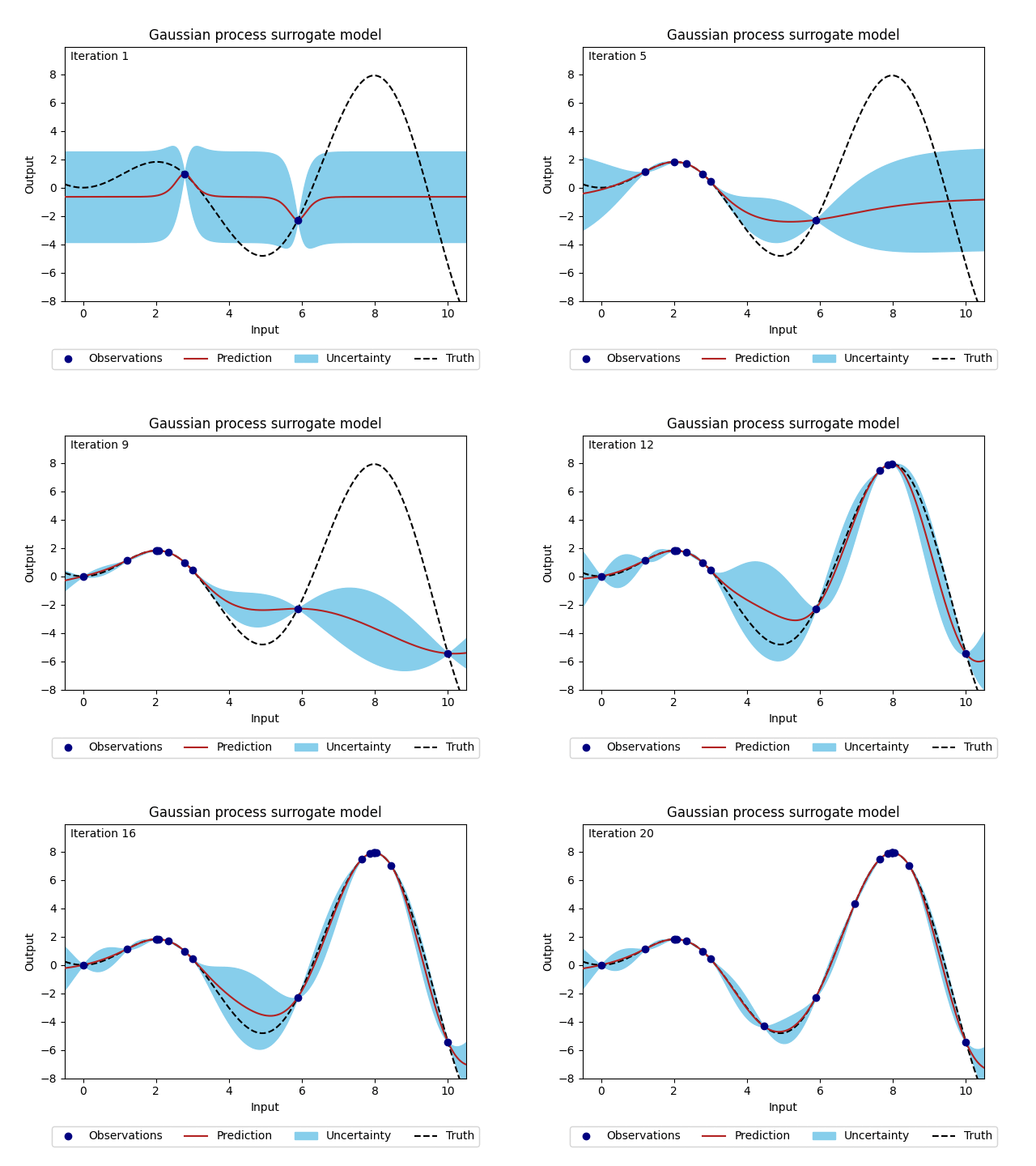
The animation below illustrates how the Bayesian optimisation algorithm works on an optimisation loop that runs for 20 iterations. The surrogate model uses the available observations to provide a prediction and its uncertainty (here shown as 95% confidence intervals around the prediction). This is our best estimate of the underlying objective function. This estimate is then used in the acquisition function to evaluate which point is most likely to improve over the current best solution. Maximising the acquisition function yields the next candidate to be observed from the objective function, before it is added to the training data and the whole process is repeated again. The animation shows how the surrogate model gets closer to the truth with each iteration and how the acquisition function explores the input space by exploring regions with high uncertainty and exploiting regions with a high prediction. This property also called the exploration-exploitation trade-off, is a cornerstone of the acquisition functions provided in NUBO.

Figure 1: Bayesian optimisation of a 1D toy function with a budget of 20 evaluations.

Surrogate model

A popular choice for the surrogate model \(\mathcal{M}\) that acts as a representation of the objective function \(f(\boldsymbol x)\) is a Gaussian process \(\mathcal{GP}\) [5] [17], a flexible non-parametric regression model. A Gaussian process is a finite collection of random variables that has a joint Gaussian distribution and is defined by a prior mean function \(\mu_0(\boldsymbol x) : \mathcal{X} \mapsto \mathbb{R}\) and a prior covariance kernel \(\Sigma_0(\boldsymbol x, \boldsymbol x') : \mathcal{X} \times \mathcal{X} \mapsto \mathbb{R}\) resulting in the prior distribution

\[f(\boldsymbol X_n) \sim \mathcal{N} (m(\boldsymbol X_n), K(\boldsymbol X_n, \boldsymbol X_n)),\]

where \(m(\boldsymbol X_n)\) is the mean vector of size \(n\) over all training inputs and \(K(\boldsymbol X_n, \boldsymbol X_n)\) is the \(n \times n\) covariance matrix between all training inputs.

The posterior distribution for \(n_*\) test points \(\boldsymbol X_*\) can be computed as the multivariate normal distribution conditional on some training data \(\mathcal{D}_n\)

\[f(\boldsymbol X_*) \mid \mathcal{D}_n, \boldsymbol X_* \sim \mathcal{N} \left(\mu_n (\boldsymbol X_*), \sigma^2_n (\boldsymbol X_*) \right)\]

\[\mu_n (\boldsymbol X_*) = K(\boldsymbol X_*, \boldsymbol X_n) \left[ K(\boldsymbol X_n, \boldsymbol X_n) + \sigma^2 I \right]^{-1} (\boldsymbol y - m (\boldsymbol X_n)) + m (\boldsymbol X_*)\]

\[\sigma^2_n (\boldsymbol X_*) = K (\boldsymbol X_*, \boldsymbol X_*) - K(\boldsymbol X_*, \boldsymbol X_n) \left[ K(\boldsymbol X_n, \boldsymbol X_n) + \sigma^2 I \right]^{-1} K(\boldsymbol X_n, \boldsymbol X_*),\]

where \(m(\boldsymbol X_*)\) is the mean vector of size \(n_*\) over all test inputs, \(K(\boldsymbol X_*, \boldsymbol X_n)\) is the \(n_* \times n\), \(K(\boldsymbol X_n, \boldsymbol X_*)\) is the \(n \times n_*\), and \(K(\boldsymbol X_*, \boldsymbol X_*)\) is the \(n_* \times n_*\) covariance matrix between training inputs \(\boldsymbol X_n\) and test inputs \(\boldsymbol X_*\).

Hyper-parameters of the Gaussian process, such as parameters \(\theta\) in the mean function and the covariance kernel and the noise variance \(\sigma^2\), can be estimated by maximising the log marginal likelihood below via maximum likelihood estimation (MLE).

\[\log p(\boldsymbol y_n \mid \boldsymbol X_n) = -\frac{1}{2} (\boldsymbol y_n - m(\boldsymbol X_n))^T [K(\boldsymbol X_n, \boldsymbol X_n) + \sigma^2 I]^{-1} (\boldsymbol y_n - m(\boldsymbol X_n)) - \frac{1}{2} \log \lvert K(\boldsymbol X_n, \boldsymbol X_n) + \sigma^2 I \rvert - \frac{n}{2} \log 2 \pi\]

Figure 2: Change of Gaussian process model (prediction and corresponding uncertainty) over 20 iterations.

NUBO uses the GPyTorch package [4] for surrogate modelling. This is a very powerful package that allows the implementation of a wide selection of models ranging from exact Gaussian processes to approximate and even deep Gaussian processes. Besides maximum likelihood estimation (MLE) GPyTorch also supports maximum a posteriori estimation (MAP) and fully Bayesian estimation to estimate the hyper-parameter. It also comes with rich documentation, many practical examples, and a large community.

NUBO provides a Gaussian process for off-the-shelf use with a constant mean function and a Matern 5/2 covariance kernel that, due to its flexibility, is especially suited for practical optimisation [13]. A tutorial on how to implement a custom Gaussian process to use with NUBO can be found in the examples section. For more complex models we recommend consulting the GPyTorch documentation.

Acquisition function

Acquisition functions use the posterior distribution of the Gaussian process \(\mathcal{GP}\) to compute a criterion that assesses if a test point is a good potential candidate point to evaluate via the objective function \(f(\boldsymbol x)\). Thus, maximising the acquisition function suggests the test point that, based on the current training data \(\mathcal{D_n}\), has the highest potential to be the global optimum. To do this, an acquisition function \(\alpha (\cdot)\) balances exploration and exploitation. The former is characterised by areas with no or only a few observed data points where the uncertainty of the Gaussian process is high, and the latter by areas where the posterior mean of the Gaussian process is high. This exploration-exploitation trade-off ensures that Bayesian optimisation does not converge to the first (potentially local) maximum it encounters, but efficiently explores the full input space.

Analytical acquisition functions

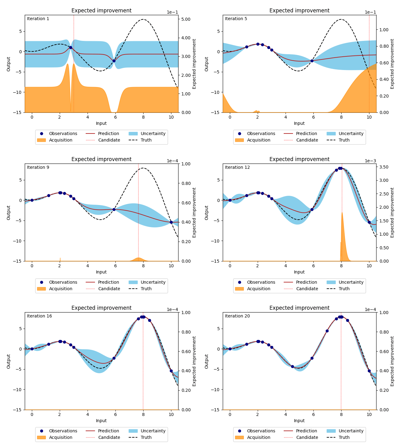
NUBO supports two of the most popular acquisition functions that are, grounded in a rich history of theoretical and empirical research. Expected improvement (EI) [6] selects points with the biggest potential to improve on the current best observation, while upper confidence bound (UCB) [14] takes an optimistic view of the posterior uncertainty and assumes it to be true to a user-defined level. Expected improvement (EI) is defined as

\[\alpha_{EI} (\boldsymbol X_*) = \left(\mu_n(\boldsymbol X_*) - y^{best} \right) \Phi(z) + \sigma_n(\boldsymbol X_*) \phi(z),\]

where \(z = \frac{\mu_n(\boldsymbol X_*) - y^{best}}{\sigma_n(\boldsymbol X_*)}\), \(\mu_n(\cdot)\) and \(\sigma_n(\cdot)\) are the mean and the standard deviation of the posterior distribution of the Gaussian process, \(y^{best}\) is the current best observation, and \(\Phi (\cdot)\) and \(\phi (\cdot)\) are the cumulative distribution function and probability density function of the standard normal distribution.

Figure 3: Bayesian optimisation using the analytical expected improvement acquisition function of a 1D toy function with a budget of 20 evaluations.

The upper confidence bound (UCB) acquisition function can be computed as

\[\alpha_{UCB} (\boldsymbol X_*) = \mu_n(\boldsymbol X_*) + \sqrt{\beta} \sigma_n(\boldsymbol X_*),\]

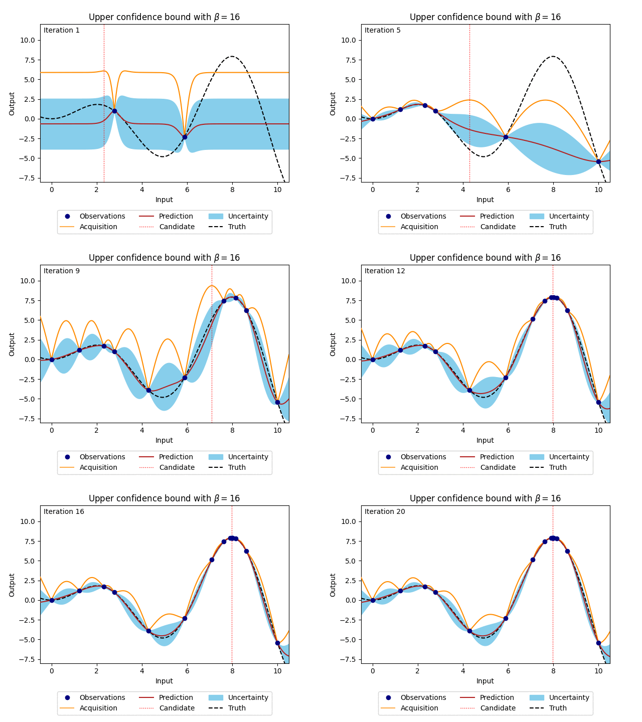
where \(\beta\) is a predefined trade-off parameter, and \(\mu_n(\cdot)\) and \(\sigma_n(\cdot)\) are the mean and the standard deviation of the posterior distribution of the Gaussian process. The animation below shows how the acquisition would look when \(\beta\) is set to 16. For comparison, the posterior uncertainty shown as the 95% confidence interval around the posterior mean of the Gaussian process is equal to using \(\beta = 1.96^2\).

Figure 4: Bayesian optimisation using the analytical upper confidence bound acquisition function of a 1D toy function with a budget of 20 evaluations.

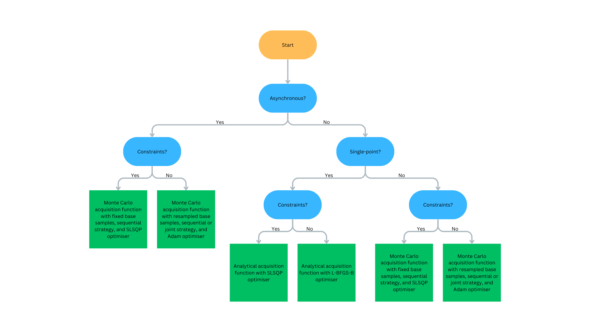
Both of these acquisition functions can be maximised with a deterministic optimiser, such as L-BFGS-B [20] for bounded and unconstrained problems or SLSQP [8] for bounded constrained problems. However, this only works for the sequential single-point problems for which every point suggested by Bayesian optimisation is observed via the objective function \(f( \boldsymbol x)\) immediatley, before the optimisation loop is repeated.

Monte Carlo acquisition functions

For parallel multi-point batches or asynchronous optimisation, the analytical acquisition functions are in general intractable. To use Bayesian optimisation in these cases, NUBO supports the approximation of the analytical acquisition function through Monte Carlo sampling [13] [18].

The idea is to draw a large number of samples directly from the posterior distribution and then to approximate the acquisition functions by averaging these Monte Carlo samples. This method is made viable by reparameterising the acquisition functions and then computing samples from the posterior distribution by utilising base samples from a standard normal distribution \(z \sim \mathcal{N} (0, 1)\).

\[\alpha_{EI}^{MC} (\boldsymbol X_*) = \max \left(ReLU(\mu_n(\boldsymbol X_*) + \boldsymbol L \boldsymbol z - y^{best}) \right)\]

\[\alpha_{UCB}^{MC} (\boldsymbol X_*) = \max \left(\mu_n(\boldsymbol X_*) + \sqrt{\frac{\beta \pi}{2}} \lvert \boldsymbol L \boldsymbol z \rvert \right),\]

where \(\mu_n(\cdot)\) is the mean of the posterior distribution of the Gaussian process, \(\boldsymbol L\) is the lower triangular matrix of the Cholesky decomposition of the covariance matrix \(\boldsymbol L \boldsymbol L^T = K(\boldsymbol X_n, \boldsymbol X_n)\), \(\boldsymbol z\) are samples from the standard normal distribution \(\mathcal{N} (0, 1)\), \(y^{best}\) is the current best observation, \(\beta\) is the trade-off parameter, and \(ReLU (\cdot)\) is the rectified linear unit function that zeros all values below 0 and leaves the rest unchanged.

Due to the randomness in the Monte Carlo samples, these acquisition functions can only be optimised by stochastic optimisers, such as Adam [7]. However, there is some empirical evidence that fixing the base samples for individual Bayesian optimisation loops does not affect the performance negatively [1]. This method would allow deterministic optimisers to be used, but could potentially introduce bias due to sampling randomness. NUBO lets you decide which variant you prefer by setting fix_base_samples and choosing the preferred optimiser. Bounded problems can be solved with Adam (fix_base_samples = False) or L-BFGS-B (fix_base_samples = True) and constraint problems can be solved with SLSQP (fix_base_samples = True).

Furthermore, two optimisation strategies for batches are possible [18]: The default is a joint optimisation approach, where the acquisition functions are optimised over all points of the batch simultaneously. The second option is a greedy sequential approach where one point after another is selected, holding all previous points fixed until the batch is full. Empirical evidence shows that both methods approximate the acquisition successfully. However, the greedy approach seems to have a slight edge over the joint strategy for some examples [18]. It is also faster to compute for larger batches. At the moment, constrained optimisation with SLSQP is only supported for the sequential strategy.

Asynchronous optimisation [13] leverages the same property as sequential greedy optimisation: the pending points that have not yet been evaluated can be added to the test points but are treated as fixed. In this way, they affect the joint multivariate normal distribution but are not considered directly in the optimisation.

Figure 5: Flowchart to determine what Bayesian optimisation algorithm is recommended. Click to expand.

---

[1]

M Balandat et al., “BoTorch: A Framework for Efficient Monte-Carlo Bayesian Optimization,” Advances in Neural Information Processing Systems, vol. 33, 2020.

[2]

M Diessner, J O’Connor, A Wynn, S Laizet, Y Guan, KJ Wilson, and RD Whalley, “Investigating Bayesian Optimization for Expensive-To-Evaluate Black Box Functions: Application in Fluid Dynamics,” Frontiers in Applied Mathematics and Statistics, 2022.

[3]

PI Frazier, “A Tutorial on Bayesian Optimization,” arXiv preprint arXiv:1807.02811, 2018.

[4]

J Gardner, G Pleiss, KQ Weinberger, D Bindel, and AG Wilson, “GPyTorch: Blackbox Matrix-Matrix Gaussian Process Inference with Gpu Acceleration,” Advances in Neural Information Processing Systems, vol. 31, 2018.

[5] (1,2)

RB Gramacy, Surrogates: Gaussian Process Modeling, Design, and Optimization for the Applied Sciences, 1st ed. Boca Raton, FL: CRC press, 2020.

[6] (1,2)

DR Jones, M Schonlau, and WJ Welch, “Efficient Global Optimization of Expensive Black-Box Functions,” Journal of Global Optimization, vol. 13, no. 4, p. 566, 1998.

[7]

DP Kingma and J Ba, “Adam: A Method for Stochastic Optimization,” Proceedings of the 3rd International Conference on Learning Representations, 2015.

[8]

D Kraft, “Algorithm 733: TOMP-Fortran Modules for Optimal Control Calculations,” ACM Transactions on Mathematical Software (TOMS), vol. 20, no. 3, p. 262-281, 1994.

[9]

OA Mahfoze, A Moody, A Wynn, RD Whalley, and S Laizet, “Reducing the Skin-Friction Drag of a Turbulent Boundary-Layer Flow with Low-Amplitude Wall-Normal Blowing within a Bayesian Optimization Framework,” Physical Review Fluids, vol. 4, no. 9, 2019.

[10]

MD McKay, RJ Beckman, and WJ Conover, “A Comparison of Three Methods for Selecting Values of Input Variables in the Analysis of Output from a Computer Code,” Technometrics, vol. 42, no. 1, p. 55-61, 2000.

[11]

J O’Connor, M Diessner, KJ Wilson, RD Whalley, A Wynn, and S Laizet, “Optimisation and Analysis of Streamwise-Varying Wall-Normal Blowing in a Turbulent Boundary Layer,” Flow, Turbulence and Combustion, 2023.

[12]

B Shahriari, K Swersky, Z Wang, RP Adams, and N De Freitas, “Taking the Human Out of the Loop: A Review of Bayesian Optimization,” Proceedings of the IEEE, vol. 104, no. 1, p. 148-175, 2015.

[13] (1,2,3,4)

J Snoek, H Larochelle, and RP Adams, “Practical Bayesian Optimization of Machine Learning Algorithms,” Advances in Neural Information Processing Systems, vol. 25, 2012.

[14]

N Srinivas, A Krause, SM Kakade, and M Seeger, “Gaussian Process Optimization in the Bandit Setting: No Regret and Experimental Design,” Proceedings of the 27th International Conference on Machine Learning, p. 1015-1022, 2010.

[15]

K Wang and AW Dowling, “Bayesian optimization for chemical products and functional materials,” Current Opinion in Chemical Engineering, vol. 36, 2022.

[16]

C White, W Neiswanger, and Y Savani, “Bananas: Bayesian Optimization with Neural Architectures for Neural Architecture Search,” Proceedings of the Aaai Conference on Artificial Intelligence, vol. 35, no. 12, 2021.

[17]

CKI Williams, and CE Rasmussen, Gaussian Processes for Machine Learning, 2nd ed. Cambridge, MA: MIT press, 2006.

[18] (1,2,3)

J Wilson, F Hutter, and M Deisenroth, “Maximizing Acquisition Functions for Bayesian Optimization,” Advances in Neural Information Processing Systems, vol. 31, 2018.

[19]

J Wu, XY Chen, H Zhang, LD Xiong, H Lei, and SH Deng, “Hyperparameter Optimization for Machine Learning Models Based on Bayesian Optimization,” Journal of Electronic Science and Technology, vol. 17, no. 1, p. 26-40, 2019.

[20]

C Zhu, RH Byrd, P Lu, J Nocedal, “Algorithm 778: L-BFGS-B: Fortran Subroutines for Large-Scale Bound-Constrained Optimization,” ACM Transactions on Mathematical Software (TOMS), vol. 23, no. 4, p. 550-560, 1997.